How do neural networks learn? A mathematical formula explains how they detect relevant patterns

Neural networks have revolutionized various fields, from image recognition to natural language processing. However, the process by which they learn to perform these tasks might seem like a black box to many. Beneath the layers of interconnected nodes lies a mathematical framework that governs how neural networks detect relevant patterns.

In this article, we’ll delve into the intricacies of neural network learning and unveil the mathematical formulas that drive their capabilities.

Neurons and Activation Functions:

Neurons serve as the fundamental building blocks of neural networks, mimicking the behavior of biological neurons in the human brain. Each neuron receives input signals, processes them, and generates an output signal. This processing is achieved through a combination of weighted sum of inputs and the application of an activation function.

In mathematical terms, let’s consider a single neuron j in a neural network layer l. The neuron receives inputs [−1]ai[l−1]​ from the previous layer, each weighted by a corresponding weight []wij[l]​. Additionally, there is a bias term []bj[l]​ associated with neuron j. The weighted sum of inputs and bias is then passed through an activation function σ, which determines the output of the neuron:

zj[l]​=σ(∑i=1n[l−1]​wij[l]​ai[l−1]​+bj[l]​)

Here, zj[l]​  represents the output of neuron j in layer l, []wij[l]​ is the weight connecting neuron i in layer −1l−1 to neuron j in layer l, [−1]ai[l−1]​ is the output of neuron i in layer −1l−1, []bj[l]​ is the bias term for neuron j in layer l, and σ is the activation function.

Activation functions introduce non-linearity into the network, enabling it to learn complex patterns in the data. They determine whether a neuron should be activated or not, based on whether the neuron’s input exceeds a certain threshold. Commonly used activation functions include:

1. Sigmoid Function: σ(z)=1+e−z1​ The sigmoid function maps the input to a value between 0 and 1, making it suitable for binary classification problems. However, it suffers from the vanishing gradient problem, which can impede training in deep neural networks.
2. Rectified Linear Unit (ReLU): σ(z)=max(0,z) ReLU is one of the most widely used activation functions due to its simplicity and effectiveness. It introduces non-linearity by outputting the input directly if it is positive, and zero otherwise. ReLU helps alleviate the vanishing gradient problem and accelerates the convergence of gradient-based optimization algorithms.
3. Hyperbolic Tangent (Tanh): σ(z)=ez+e−zez−e−z​​ Tanh function is similar to the sigmoid function but maps the input to a value between -1 and 1. It is often used in hidden layers of neural networks, offering stronger gradients compared to the sigmoid function.

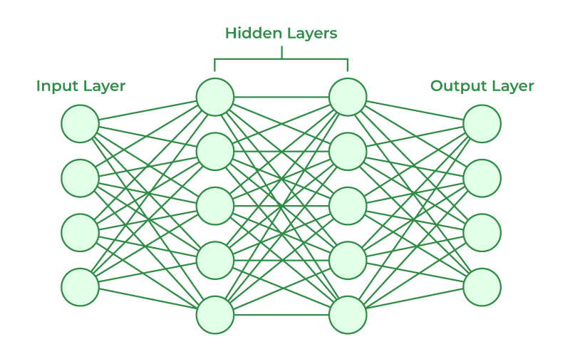
To illustrate, consider a simple neural network with one input layer, one hidden layer with two neurons, and one output layer. Each neuron in the hidden layer receives inputs from the input layer, applies the activation function, and passes the output to the output layer. The output layer produces the final prediction based on the inputs from the hidden layer. This process of weighted sum computation followed by activation is repeated across the network, allowing it to learn and generalize from the data.

Example:
Let’s consider a simple neural network tasked with classifying images of handwritten digits into one of ten classes (0 through 9). The input to the network is a grayscale image of size 28×28 pixels, resulting in 784 input neurons. The network has one hidden layer with 100 neurons and an output layer with 10 neurons (one for each class).

During the forward pass, each neuron in the hidden layer receives inputs from all neurons in the input layer, computes a weighted sum of inputs, and applies an activation function such as ReLU. The output of the hidden layer neurons then becomes the input for the neurons in the output layer, which apply another activation function such as softmax to produce the final probabilities for each class.

By iteratively adjusting the weights and biases of the neurons using techniques like backpropagation and gradient descent, the network learns to accurately classify handwritten digits based on the input images.

Forward Propagation:

Backpropagation:

Backpropagation is a fundamental algorithm in training neural networks. It enables the adjustment of the network’s parameters (weights and biases) based on the computed gradients of the loss function with respect to these parameters. By propagating the error backward through the network, backpropagation allows for efficient optimization of the network’s performance.

The backpropagation algorithm consists of two main steps:

1. Forward Pass: During the forward pass, input data is passed through the neural network, layer by layer, to produce a prediction at the output layer. The output is computed using the network’s current parameters (weights and biases) and activation functions. The output is then compared to the true labels using a loss function, which quantifies the discrepancy between the predicted and actual outputs.
2. Backward Pass: In the backward pass, the gradients of the loss function with respect to the parameters of the network are computed using the chain rule of calculus. These gradients indicate how the loss would change with small changes in each parameter. The gradients are then used to update the parameters in a way that reduces the loss, thereby improving the network’s performance.

Example:
Let’s consider a simple neural network with one input layer, one hidden layer, and one output layer. The network is trained to perform binary classification, with two classes (0 and 1).

During the forward pass, input data is passed through the network, and the output is computed using the current parameters. Let’s say the output is 0.7, indicating a probability of 0.7 for class 1.

Next, during the backward pass, the gradients of the loss function with respect to the parameters are computed. These gradients indicate how the loss would change with small changes in each parameter. The gradients are used to update the parameters (weights and biases) in a way that reduces the loss.

For example, if the true label is 1, the loss function might be binary cross-entropy loss. The gradients are computed based on the difference between the predicted output (0.7) and the true label (1), and the parameters are updated accordingly to reduce this difference in subsequent iterations.

Through repeated forward and backward passes, the network gradually learns to better classify the input data, adjusting its parameters to minimize the loss and improve its performance.

 

Gradient Descent:

Gradient descent is an optimization algorithm used to minimize the loss function of a neural network by iteratively adjusting its parameters (weights and biases). It works by computing the gradient of the loss function with respect to each parameter and updating the parameters in the opposite direction of the gradient.

The gradient points in the direction of the steepest increase in the loss function. Therefore, by moving in the opposite direction of the gradient, we can descend along the loss function towards a minimum.

There are several variants of gradient descent, including batch gradient descent, stochastic gradient descent (SGD), and mini-batch gradient descent. Each variant differs in how it computes the gradients and updates the parameters.

1. Batch Gradient Descent: In batch gradient descent, the gradients of the loss function with respect to all parameters are computed using the entire training dataset. The parameters are then updated once per iteration using the average gradient across all samples. Batch gradient descent can be computationally expensive for large datasets since it requires computing gradients for the entire dataset at each iteration.
2. Stochastic Gradient Descent (SGD): In stochastic gradient descent, the gradients of the loss function are computed using only one training sample at a time. The parameters are updated after computing the gradient for each sample. SGD can be faster than batch gradient descent since it updates the parameters more frequently. However, the updates can be noisy and may oscillate around the minimum.
3. Mini-Batch Gradient Descent: Mini-batch gradient descent is a compromise between batch gradient descent and SGD. It computes gradients using a small subset of the training data called a mini-batch. The parameters are updated once per mini-batch. Mini-batch gradient descent combines the advantages of batch gradient descent (stable convergence) and SGD (faster updates).

The update rule for gradient descent is given by:

θ=θ−α∇J(θ)

Where:

• $\theta$ represents the parameters of the neural network (weights and biases).
• $J(\theta )$ is the loss function.
• $\nabla J(\theta )$ is the gradient of the loss function with respect to the parameters.
• $\alpha$ is the learning rate, which controls the size of the parameter updates.

The learning rate is a hyperparameter that needs to be carefully chosen. A high learning rate may cause the algorithm to diverge, while a low learning rate may lead to slow convergence.

Example: Consider training a neural network for image classification using mini-batch gradient descent. At each iteration, a mini-batch of training samples is randomly selected from the dataset. Forward propagation is performed to compute the output of the network for each sample in the mini-batch. Then, the loss function is computed based on the predicted outputs and the true labels.

Next, the gradients of the loss function with respect to the parameters (weights and biases) are computed using backpropagation. Finally, the parameters are updated using the gradients and the learning rate according to the gradient descent update rule.

This process is repeated for multiple epochs until the parameters converge to values that minimize the loss function and optimize the performance of the neural network.

Conclusion:

Neural networks operate by combining the functionalities of neurons and activation functions across multiple layers to solve complex problems in various domains. The process involves several key steps:

1. Input Processing: Input data is fed into the neural network, typically in the form of features extracted from raw data. These features are passed through the input layer, where each neuron receives and processes specific input signals.
2. Hidden Layer Computations: The input signals are then transformed through a series of hidden layers, each consisting of neurons that perform weighted sums and apply activation functions. These transformations allow the network to learn intricate patterns and relationships within the data.
3. Output Generation: The output layer produces the final output of the network, which could be predictions for a classification task or numerical values for a regression task. The output is computed based on the processed information from the hidden layers and is typically passed through an appropriate activation function.
4. Loss Calculation: The predicted output is compared to the ground truth labels using a loss function, which quantifies the discrepancy between the predicted and actual outputs. The goal during training is to minimize this loss function by adjusting the parameters (weights and biases) of the network.
5. Optimization through Backpropagation: Backpropagation is employed to compute the gradients of the loss function with respect to the parameters of the network. These gradients guide the optimization process, allowing the network to update its parameters in a way that reduces the loss and improves performance.
6. Gradient Descent: Gradient descent algorithms, such as stochastic gradient descent or mini-batch gradient descent, are used to iteratively update the parameters of the network based on the computed gradients. By descending along the loss function, the network converges towards optimal parameter values that minimize the loss.

Through the collective operation of these components, neural networks are capable of learning complex patterns, making accurate predictions, and solving a wide range of tasks including image recognition, natural language processing, and speech recognition. The ability to automatically extract meaningful representations from raw data and generalize to unseen examples makes neural networks powerful tools for tackling real-world problems across various domains.